WolvWatch
Building a custom smartwatch — from the ground up.
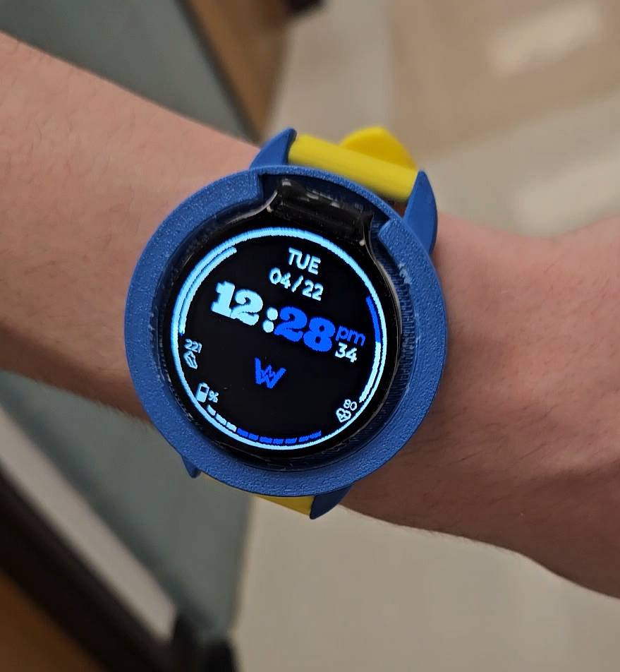
Ever wondered what goes into a smartwatch? This past semester (Winter 2025), my EECS 373: Intro to Embedded Systems team decided to find out.
Over the final month and a half of the semester, we developed, fabricated, and tested an entirely custom smartwatch, integrating features typically found in commercial-grade products.
This post serves as a comprehensive breakdown of this project, including technical details, organizational and logistical challenges, and a reflection. Feel free to skip around to points of interest using the sidebar!
System Architecture
Before getting into specifics, let’s outline the high-level design. We aimed for a classic smartwatch architecture: central microcontroller (MCU) connected to various peripherals (display, sensors, buttons) all powered by a small lithium polymer (LiPo) battery.
- Microcontroller: STM32L496RGTx
- Display: 1.28” circular 240x240 pixel TFT LCD with an integrated GC9A01 LCD driver
- Connectivity: HC-05 bluetooth module
- Sensors:
- MAX30102 heart rate / SPO2 sensor
- ADXL362 accelerometer
- Power: 300mAh 1S LiPo battery
- Input: three side buttons (up, enter, down)
Display
Communicating over SPI
The LCD driver utilizes the Serial Peripheral Interface (SPI) communication protocol. I’m going to skip over the setup sequence of commands needed to get the display into a working state, but if you’re interested feel free to check out the associated source code.
The driver provides several different modes, but for our purposes we used RGB565. The numbers here define the number of bits used to represent each of the three additive primary colors:
- Red: 5 bits
- Green: 6 bits
- Blue: 5 bits
Each pixel is then represented by two bytes (16 bits) rather than the typical three byte model (for example HEX codes like #FFFFFF). This means that the buffer used to store the state of the screen is smaller, but it also means that we can’t represent as many colors. This tradeoff was perfectly fine for our needs, however. In fact, when dealing with ultra-tight memory constraints on our first iteration we actually started using RGB111 (i.e. one bit per color, only eight colors total) to save a bit of space!
These color values are sent over the SPI communication lines in a “burst” write column-by-column and row-by-row.
Drawing to the Screen
The method we ultimately chose for this task is the frame buffer approach, where you store the state of the screen (i.e. the color of each pixel) directly in memory, and periodically push it to the hardware to be displayed to the user.
The main drawback with this approach is its constant, large memory usage. Using our setup as an example, each pixel is represented by two bytes of data. There are $240\cdot240=57,600$ pixels, which when multiplied by 2 bytes/pixel results in a memory overhead of $115\text{ kB}$. That is a huge amount of memory in the world of embedded systems. Our first iteration, for instance, had only $64\text{ kB}$ of total memory capacity.
However, where this method shines is in its speed and simplicity. Here’s the main bit of code that drives the screen:
1
2
3
4
5
6
7
8
9
10
11
12
13
14
15
16
17
18
19
20
21
22
23
24
25
26
27
28
29
30
31
32
33
34
35
36
static uint16_t pixels[LCD_1IN28_HEIGHT][LCD_1IN28_WIDTH]; // pre-allocated two-dimensional array to hold the pixel values of the entire screen

// sets a given pixel to a specific color
void screen_set_pixel(uint16_t x, uint16_t y, uint16_t color) {
    pixels[y][x] = color;
}

// sends the current buffer to the physical screen
void screen_render() {
    // tell the LCD driver that we're editing pixels (0,0) to (239, 239)
    // i.e. we're editing the entire screen
    screen_set_windows(0, 0, 239, 239);

    SET_DC_HIGH;
    SET_CS_LOW;

    /*
     * This is the main linkage between our code and the physical screen.
     * The hardware on the STM32 used to send data to the screen can only handle 65536 ($2^16-1$) bytes at once,
     * thus our code "chunks" the buffer into multiple pieces that the underlying hardware can then handle.
    */
    uint32_t bytes_remaining = 240 * 240 * 2;
    uint32_t offset = 0;
    while (bytes_remaining > 0) {
        if (bytes_remaining > 65000) {
            HAL_SPI_Transmit(&hspi3, (uint8_t *) pixels + offset, 65000, HAL_MAX_DELAY);
            offset += 65000;
            bytes_remaining -= 65000;
        } else {
            HAL_SPI_Transmit(&hspi3, (uint8_t *) pixels + offset, bytes_remaining, HAL_MAX_DELAY);
            bytes_remaining = 0;
        }
    }
    SET_DC_LOW;
    SET_CS_HIGH;
}
Rasterization
Great, so now we have a mechanism to set specific pixels to specific colors! But how do we get useful things onto the screen like shapes, text, and images? This is where the concept of rasterization comes in. The concept refers to taking an image in some vector graphics format, and translating that into pixel values on a screen. In this blog, however, I’m using it to refer to the general process of operating on any shape, including text.
Shapes
The task of shape rasterizing is a lot more involved than we initially thought, and as such the code is a bit long to include here, but if you’re interested check out the relevant source code. Essentially, we used Xiaolin Wu’s line algorithm and then used that as a basis to create other shapes.
Text
Most people probably don’t think twice about how text is rendered behind the scenes, as the operating system carries the brunt of this work. Now, remove that operating system, and you have a bit of a problem! There is no built-in mechanism to parse standard font files, so we had to do something a bit different. We used a program called LCD Image Converter to take the fonts and convert them to a bitmap that then gets stored as static data in a C header.
Your next question may be “well what the hell is a bitmap?” Basically, an image is converted into a bitmap by first “flattening” it (taking each row and placing it after the last, essentially turning the image into a one-dimensional line) and then iterating over the pixels in order, mapping black to 0 and white to 1. You could use more colors than this, but since we were memory constrained and were only rendering text, we used a monochrome one-bit color scheme.
As I said earlier, this data is then turned into a single array that can be iterated over by the program to recreate the image on the LCD.
Sensors
MAX30102 Heartrate Sensor
The heartrate sensor was one of the more difficult aspects of this project. The manufacturers provided a plug-and-play library, however after some initial testing we quickly realized that the output was far too noisy, so we decided to take on the challenge of writing our own firmware to process the raw data!
How does a heartrate sensor work?
At a high level, a heartrate sensor is essentially just a light attached to a light detector. If you’ve ever seen one of those phone apps that allows you to get your heartrate by placing your finger over your flashlight+camera, then you’ve seen this mechanism in action. The amount of light reflected back changes alongside blood volume within capallaries, with correlates with heart rate. If you’d like to read up on it in more depth, the formal term is photoplethysmography.
Filtering
Data from virtually any sensor is going to be subject to noise from the environment, and it’s important to remove as much of this as possible without significantly affecting the components of the data you do want. Luckily for me, while working on this project I was also enrolled in a Signals and Systems course, which is in part concerned with this very topic! Ultimately, I decided to use a fourth-order butterworth filter alongside the internal sample averaging that the heartrate chip has on-board.
The basic principle of a butterworth filter is that it’s a bandpass filter, i.e. it lets through only a specific band of frequencies and rejects all others. I derived the band required for this sensor by taking the lowest and highest heartrate we’d reasonably see, and converted the beats/minute into hertz. We chose 60bpm and 200bpm as our low and high respectively, which translates to an approximate band (in hertz) of [1, 3.33], which is what we then used in the butterworth filter.
Signal Processing
Now that we had a fairly clean signal to work with, we needed to actually count the beats! This is done with a peak detection algorithm, which looks for local maxima in a predefined window of time. Essentially, we look at the last 10 seconds or so, then ask “how many high points do we see?” and divide that by 10 to get the beats per second (which can then be multiplied by 60 to get beats/min). We used an algorithm similar to the one MatLab uses.
Here’s a screenshot of what this actually looked like when we were testing: 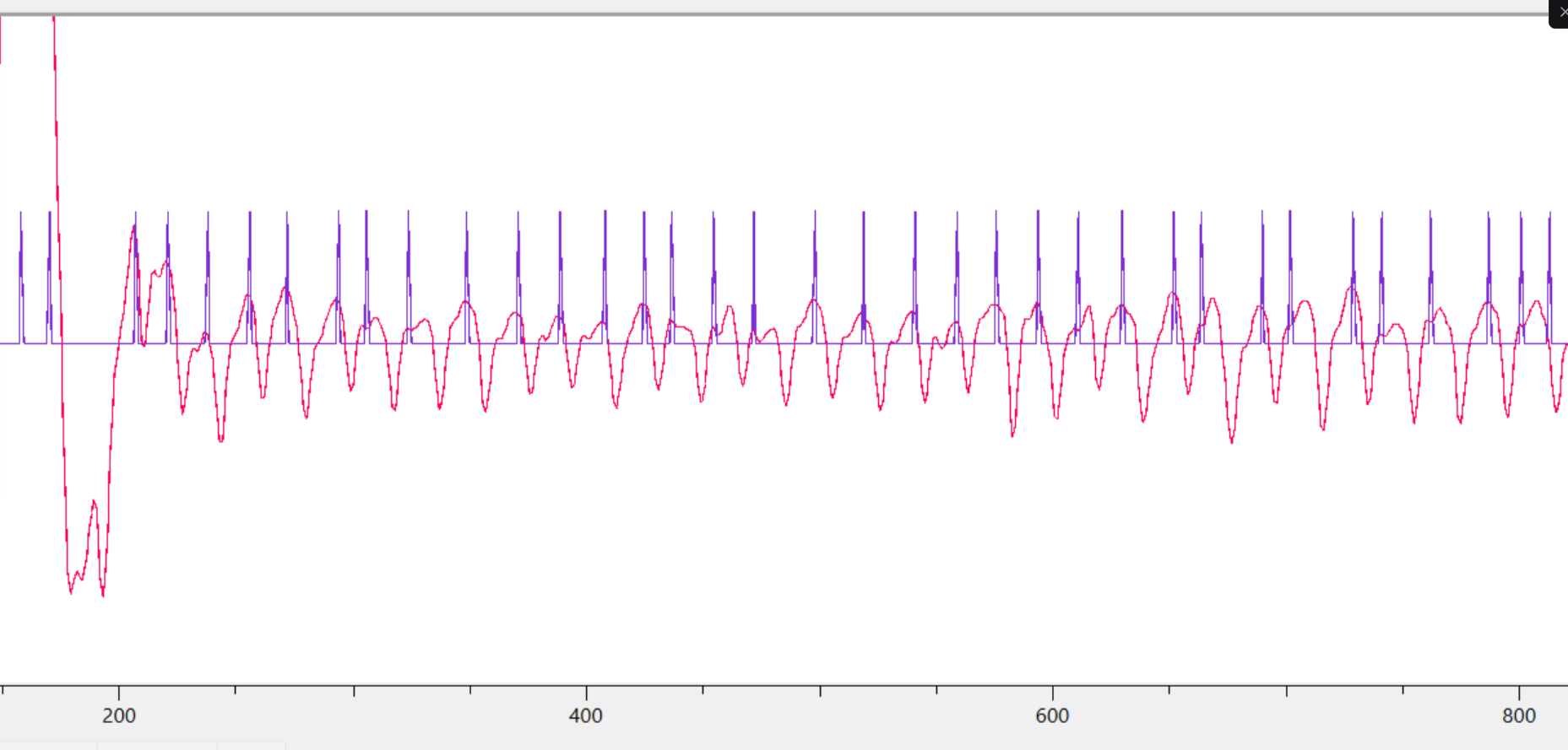
The red line is the filtered sensor data, and each blue peak represents a detected heartbeat. Pretty cool, huh?
ADXL362 Accelerometer
Originally our plan was to implement both step counts and a raise-to-wake feature, but we ran out of time for the latter. Luckily, Analog Devices (the manufacturer of the chip we used) had a guide for implementing a step-counting algorithm on a similar model, so we used that as our foundation and modified it to work with our setup. You can read the guide we used here.
The basic idea behind this is actually very similar to how we detected heartrate: look at a predefined window of time, count how many local maxima (peaks) are in the data, and add them to the running total. The main difference is the frequency band we’re looking at, since the average human walks/runs between 0.5 Hz and 2 Hz.
There is also a slight addition: we want to avoid false counts when moving around but NOT walking. The way we accomplish this is by requiring 8 step counts in a specific period of time before entering “walking” mode and counting steps continually. If we don’t reach this required number of steps, the data is discarded, as it’s likely we’re not actually walking and may just be moving our arms around.